A side objective#
A few months ago, I developed a framework to learn about good software architecture design in C++ for simulations. As a test case, I chose 2D diffusion. One simulation used random walkers, while another used the discretised version of the diffusion equation. Two fundamentally different simulation methods, yet they model the same phenomenon. Understanding why this is the case is an interesting topic in itself, and worthy of its own post.
The simulation framework#
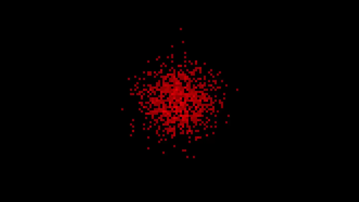
The above video is the output of the 2D diffusion simulation framework using random walkers. Each red pixel is a random walker. The greater the concentration of walkers, the redder the pixel.
A random walker is a particle set to move in a random direction at every time step. In this simulation, each walker moves independently, with equal probability in every direction.
This approach belongs to a broader category of techniques known as Monte Carlo methods. These methods use randomness to approximate what could be solved deterministically. In this case, instead of using the diffusion equation directly, we get diffusion through the statistical output of many random walkers.
Contrast this with the video below. This output comes from numerically solving the diffusion equation:
$$ \frac{\partial \rho}{\partial t} = D \left( \frac{\partial^2 \rho}{\partial x^2} + \frac{\partial^2 \rho}{\partial y^2} \right) $$where \(D\) is the diffusion coefficient, and \(\rho\) is the concentration at point \((x, y)\) for a given time \(t\).
Rather than moving particles randomly, the same system is represented as a grid of concentration values, one at each point in space.
Now, we have to ask ourselves, is what we are seeing in both simulations truly what ideal diffusion predicts?
Visually, both methods appear to show diffusion, but to be sure they simulate ideal diffusion, we need a quantitative measure.
There is one key property of diffusion that we can easily measure: the average squared distance of the distribution from the starting point, the mean squared displacement, grows proportionally with time.
By measuring the mean squared displacement, we can quantitatively compare the random walk and the numerical method.
A basic comparison#
For the random walk simulation, after each time step, we measure how far each walker is from the origin by squaring its displacement and summing them. For example, if \(x_i\) and \(y_i\) are the \(x\) and \(y\) positions of the \(i^{\text{th}}\) walker, we do:
$$ \sum_{i}^N \left((x_i - x_0)^2 + (y_i - y_0)^2\right) $$where \(N\) is the total number of walkers and \(x_0\) and \(y_0\) are the origin positions.
If we did not square the displacements, then positive and negative displacements would cancel along the same axis. We are calculating how far the distribution spreads out from the origin; the direction shouldn’t matter. This value is then averaged across all walkers at the same time step to get:
$$ \frac{1}{N}\sum_{i}^N \left((x_i - x_0)^2 + (y_i - y_0)^2\right) $$We repeat this process at every step to track how the spread evolves over time.
The same idea is applied in the numerical simulation. However, each grid point contributes both its distance from the origin and the concentration at that point. This means that after squaring the distance, we multiply it by the concentration at that same point. This acts like a weighting factor, so regions with more concentration influence the result more strongly:
$$ \frac{\sum_{x,y} \rho_{x,y}\left((x - x_0)^2 + (y - y_0)^2\right)}{\sum_{x,y} \rho_{x,y}} $$Notice how we have \(\sum_{x,y} \rho_{x,y}\) instead of \(\frac{1}{N}\) in this case.
If we plot these measurements against time for each simulation method, we see that both follow a linear relationship. This is a defining property of ideal diffusion: the spread increases steadily rather than accelerating or slowing down, assuming there are no boundaries.
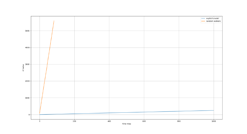
Clearly the slopes differ, however, this is due to differing initial conditions. In this case, the random walkers are set to travel at a greater distance per time step than what the diffusion coefficient of the equation model allows.
So how is it that particles in random motion are able to approximate diffusion?
The diffusion model#
The Monte Carlo random walk and diffusion model are not independent. In fact, we can derive the diffusion equation from the random motion of a particle.
My simulation framework moves the random walkers continuously and then locks them into a discrete grid. For simplicity, we’ll assume the random walkers move discretely instead. In other words, we’ll assume this instead:
direction = getRandomDirection()

if (direction == "Left") : particleMoveToLeftCell()
if (direction == "Right") : particleMoveToRightCell()
if (direction == "Up") : particleMoveToTopCell()
if (direction == "Down") : particleMoveToBottomCell()
Let’s assume a random walker lives on the following grid:
We’ll highlight the following region and make it our focus:

Suppose we wanted to work out the probability of the walker being in \((x,y)\) at time \(t + \Delta t\):

We know that the probability of where the walker is now depends on where it was before. We know it could only have been in the left, right, top or bottom cell, at time \( t \).

This means, from any one of those neighbouring cells, there is a \(\frac{1}{4}\) chance of a walker entering \(x, y\) at time \(t + \Delta t\).
This gives an equation we can start with:
$$ P_{x,y}(t + \Delta t) = \frac{1}{4}(P(\textbf{left cell } \text{OR } \textbf{right cell } \text{OR } \textbf{top cell } \text{OR } \textbf{bottom cell })) $$However, we know the walker could only have been in one of those four positions at time \( t \), but not all of them at once. In other words, all four possible positions are mutually exclusive:
$$ P(\textbf{left cell } \text{OR } \textbf{right cell } \text{OR } \textbf{top cell } \text{OR } \textbf{bottom cell }) = P_{x-1,y}(t) + P_{x+1,y}(t) + P_{x,y-1}(t) + P_{x,y+1}(t) $$This gives us the following equation:
$$ P_{x,y}(t + \Delta t) = \frac{1}{4}\left(P_{x-1,y}(t) + P_{x+1,y}(t) + P_{x,y-1}(t) + P_{x,y+1}(t)\right) $$We want to convert this into the partial differential equation of the diffusion model. We know this implies a difference between two points. So let’s subtract \(P_{x,y}(t)\) from both sides:
$$ P_{x,y}(t + \Delta t) - P_{x,y}(t) = \frac{1}{4}( P_{x+1,y}(t) + P_{x-1,y}(t) + P_{x,y+1}(t) + P_{x,y-1}(t) - 4P_{x,y}(t)) $$The \(4P_{x,y}(t)\) term in the right hand side cancels the \(\frac{1}{4}\).
Currently, the equation is unitless. However, we can divide the left hand side by the time step to convert into probability per unit time, and the right hand side by the \(\Delta x^2 \) and \(\Delta y^2 \) to convert into probability per unit length squared:
$$ \frac{P_{x,y}(t + \Delta t) - P_{x,y}(t)}{\Delta t} \Delta t = \frac{1}{4}\left( \Delta x^2 \frac{P_{x+1,y}(t) -2P_{x,y}(t) + P_{x-1,y}(t)}{\Delta x^2} + \Delta y^2\frac{P_{x,y+1}(t) - 2P_{x,y}(t) + P_{x,y-1}(t)}{\Delta y^2}\right) $$You may have noticed that:
$$\frac{P_{x+1,y}(t) -2P_{x,y}(t) + P_{x-1,y}(t)}{\Delta x^2}$$and
$$\frac{P_{x,y+1}(t) - 2P_{x,y}(t) + P_{x,y-1}(t)}{\Delta y^2}$$are the discrete approximations for the second derivatives, \(\frac{\partial^2 P}{\partial x^2} \) and \(\frac{\partial^2 P}{\partial y^2} \).
Similarly,
$$ \frac{P_{x,y}(t + \Delta t) - P_{x,y}(t)}{\Delta t} $$is the discrete approximation for \(\frac{\partial P}{\partial t} \).
If we take the limit of \(\Delta t\), \(\Delta x\) and \(\Delta y\) in the fractions as they approach \(0\), we can rewrite the equation as:
$$ \frac{\partial P}{\partial t} \Delta t = \frac{1}{4}\left(\Delta x^2 \frac{\partial^2 P}{\partial x^2} + \Delta y^2\frac{\partial^2 P}{\partial y^2}\right) $$Dividing by \(\Delta t\) on both sides we get:
$$ \frac{\partial P}{\partial t}= \frac{\Delta x^2}{4 \Delta t} \frac{\partial^2 P}{\partial x^2} + \frac{\Delta y^2}{4 \Delta t}\frac{\partial^2 P}{\partial y^2} $$In this case, the diffusion coefficient is split into two:
$$ D_x = \frac{\Delta x^2}{4 \Delta t} $$and
$$ D_y = \frac{\Delta y^2}{4 \Delta t} $$However, \(\Delta x\) and \(\Delta y\) are often made equal, such as in my simulation framework, and so we can set:
$$ D = D_x = D_y $$to get:
$$ \frac{\partial P}{\partial t}= D\left(\frac{\partial^2 P}{\partial x^2} + \frac{\partial^2 P}{\partial y^2}\right) $$Look familiar?
We’ve derived a model for a real-world thermodynamic process, all from the random and independent motion of particles.
More on diffusion#
Ultimately, diffusion occurs from the kinetic collisions of an unimaginable number of particles. Naturally, this leads to particles spreading out over time as they occupy areas with fewer particles. The diffusion equation we calculated and use represents the overall concentrations of the particles, not their individual collisions.
In fact, with enough particles, we’ve shown that a random walk can approximate the average net displacement of diffusing particles.
Statistically based simulations, such as the random walk, are useful for efficiently solving systems where a deterministic solution is more difficult or computationally expensive. That’s where Monte Carlo simulations, such as the random walk, are particularly useful.
Article Resources#
Diffusion simulation framework github